Uncovering local property tax evasion using machine learning and statistical modeling. An investigative recipe.
If there's one universal investigative template I've come across in my journalism career, it's this: take a list of names or organizations, find those names in another dataset[1] and identify the most suspicious ones for further investigation. I call this a "data in, data out" investigation. While I've personally only applied this pattern to property tax related stories, it could also be extended to areas like campaign finance and background research.
Before I get into the technical dirt, I want to talk about why data in, data out investigations are ideal. Going into a dataset essentially blind and letting the data provide leads helps keep things less biased. Smaller newsrooms can benefit, too, because they don't need whistleblowers telling them exactly who or what to look for. To me, the best part is these kinds of investigations lend themselves well to advanced computer assisted methods—eliminating a lot of the tedium that goes into investigative work.
I'm going to dissect a data in, data out investigation and the machine learning (ML)[10] tools that went into it.
The City of Austin, like many cities across the US, requires people who list their homes on sites like HomeAway and Airbnb to register and pay taxes on each stay, just like hotels do. These types of rentals are called "short-term rentals" (STRs). Properties used as STRs generally aren't eligible for most tax exemptions. In Texas, home owners can apply for a so-called "homestead exemption". These add up to significant tax savings. Because of this, there are lots of rules around them. For example, only one property per person or couple can be exempt. It needs to be their primary residence and it can't be used commercially.
We wanted to see whether the appropriate rental taxes were being paid and if the appraisal district was letting STR operators apply for and receive tax exemptions—a clear violation of the law.
A list of STRs registered with the city was the primary dataset. Secondarily, we got datasets of appraisal district properties and electric utility subscribers. We took the STR list and used a ML algorithm to look for matches in the other two datasets. This identified STR operators (individuals or couples) who owned multiple properties and had applied for exemptions.
Next, we checked each joint STR/property record for exemptions and ranked them by suspiciousness. This ranking was accomplished using ML. From there, we filed a series of public information requests to verify our findings.
Joining two datasets based on one of their columns is a basic strategy common to many investigations. Relational databases were created to do exactly this. But in our case, we had low quality data and a lot of it: roughly a million records, combined. Names were spelled inconsistently and addresses were often abbreviated or were missing apartment numbers. Standard tools didn't cut it, so we turned to ML.
The foundation of my approach to this investigation is a ML algorithm called Locality Sensitive Hashing (LSH). This is part of the unsupervised[19] machine learning family of algorithms. Unsupervised learning gets its name because it learns directly from the data itself. Unlike other forms of ML, unsupervised methods don't require people to tediously sort through data and tag individual records. These algorithms are inexpensive to use, can work in a variety of situations and lend themselves to straightforward, practical applications. Unsupervised learning excels in problems like search, uncovering structure, similarity, grouping and segmentation. It's my opinion that unsupervised machine learning holds the most promise for the future of local and nonprofit investigative journalism.
LSH is an algorithmic method for taking large amounts of data and efficiently grouping together records which are similar to each other. It can handle inexact or "fuzzy" matches, greatly reducing the amount of preprocessing[8] needed.

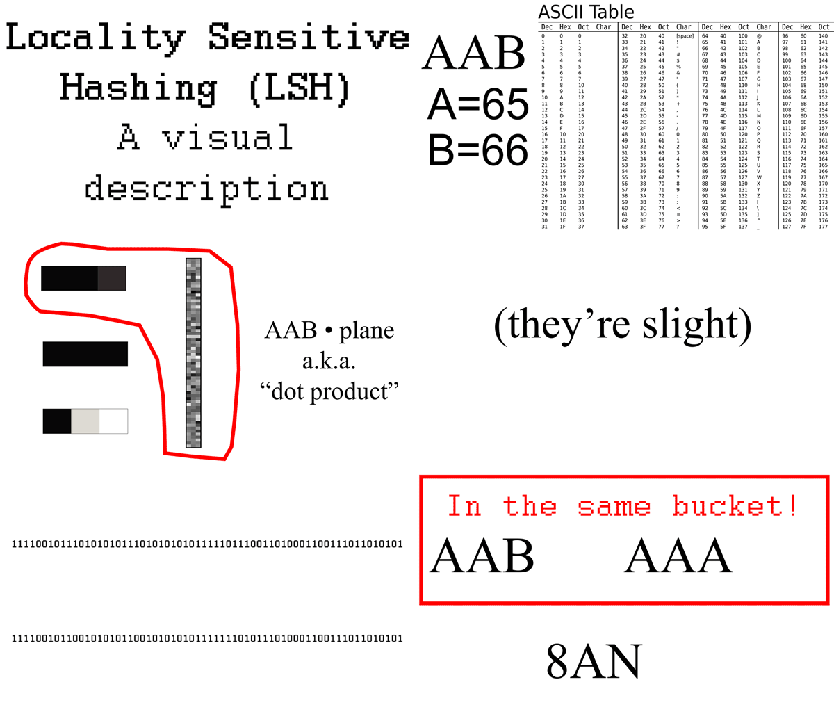
An animation of the process of grouping three short random words into groups using LSH.
In short, LSH operates by taking data points and assigning them to "buckets" or groups. When using LSH to link records from two datasets, we take the larger dataset, build an LSH index and then take the smaller dataset and query that index. The result of a query is a list of records which should be similar to the record we're querying.
I'm going to give a technical overview of the specific LSH algorithm I used. Feel free to skip this part if you don't care.
--------------- START TECHNICAL DISCUSSION ---------------
In order to understand LSH, we first need to discuss the k-Nearest Neighbors (k-NN) algorithm. What k-NN does is take one set of records and allow you to find some number of most similar records. That number is the k in k-NN. So a k-NN algorithm that only finds the single most similar record is known as k-NN with k=1 or (sometimes) 1-NN. In its most basic form, this algorithm checks every point against each other and gets a score for how similar they are. We then rank these and take the k-number of closest matches. While this algorithm has its place, it is problematic in our investigation for several reasons:
- I had a dataset of 20,000 properties and another dataset of 800,000 utilities records. Doing the math, 20,000 records times 800,000, tells us 16,000,000,000 checks need to be performed to find groups using plain old k-NN.
- Even if doing that number of checks was feasible, I'd need to come up with a distance[2] threshold—a number that establishes how similar two records need to be in order to be considered the same.
Both of these problems are annoying to solve and can be avoided by using LSH, which is a form of approximate nearest neighbors.
LSH goes about finding similar records using what I mentally categorize as a mathematical cheat code: if two records, A and B, are similar to a third record, then the two are likely similar to each other. It's a massive simplification of how LSH works, but it serves as a decent mental model. This gets around having to check every record against every record in order to find groups. We only need to check all records against that third thing.
In reality, LSH works by projecting[9] our records onto a randomized hyperplane (basically a random matrix[11]
of data), doing a little rounding, and assigning them to a bucket. The smaller the hyperplane is, the higher chance that records will end up in the same bucket, despite dissimilarity.
Generally, this is a lot quicker than k-NN because, for each record, we only need to do a multiplication with the hyperplane. Mathematically speaking, LSH scales linearly with the number of records, as opposed to k-NN which scales exponentially. In my example above of 20,000 and 800,000 records, I only need to do 820,000 checks (800,000 plus 20,000 checks against our hyperplane). Obviously, this is far less than the 16,000,000,000 checks with plain k-NN.
--------------- END TECHNICAL DISCUSSION ---------------
Grouping records in LSH is done probabilistically, meaning you probably won't find every match and some non-matches might also fall into your results. Fortunately, there are ways to tune LSH in order to avoid this. LSH has two main configuration options, if you will. The most important being the hash[5] size. The larger the hash size, the more similar records must be to end up in the same bucket. Another way to improve accuracy is to use multiple LSH indexes. This increases the chances of records falling into the same bucket if they are indeed similar. I tend to use three LSH indexes with a hash size of either 512 or 1024 bits. (Another strategy for finding a good hash size is to start with the square root of the number of records and go up from there. Wikipedia has a decent page on this.)
The process for grouping records between two datasets using LSH goes like this:
- Choose a column to match records with and extract that column from each dataset (e.g., we want to match against owner name, so get the "owner name" column from one dataset and "name" on the other).
- Take only one of our extracted columns for matching and build a LSH index with it (e.g., build a LSH index on the "owner name" column).
- Take the second, remaining column and query (get bucket assignments from) our LSH index (e.g., for each value in the "name" column, get the most similar names from the "owner name" column). The results of each query forms a "group" of similar records.
- For each match in each group, grab the original full record. We will use the combined group of records to continue our investigation.
This process results in a list of grouped records. I tend to flatten these groups into wide rows by combining fields from both datasets. I also add some extra columns describing things like the number of matches found in the bucket and some averages from the records. We can use this data to filter out groups that aren't worth investigating further and then rank the remaining records by investigative interest. But instead of doing this last step by hand, I propose using another ML technique: regression.
So, we've successfully identified groups of records and now want to uncover ones that warrant intensive, manual research. We've also built a few aggregates from each group to work with. In the investigation described above, we had these aggregate variables (or features[4]) to work with:
- Number of properties owned.
- Total number of exemptions held.
- Total monetary amount of combined exemptions.
- Property type (there were three types of properties, with different rules about how exemptions may legally be applied).
- Average valuation of all properties owned.
Typically, one might consider writing a program to take these values and use them to rank grouped records. We could do this by assigning an importance value, or weight[21], to each variable, combining them and obtaining a score for each group.
This may sound good, but there are still some open questions. How do we combine the variables for each group? How do we compare variables with different ranges? The valuation of a property, for example, is in the hundreds of thousands, while the number of exemptions applied to a property is in the single digits. How do we combine everything once we've decided on importance? What do we do if some of the variables are redundant and overpower other, more important, variables? Luckily there is ML algorithm that can help with all of these problems.
Regression is a statistical modeling technique in the supervised[17] family of ML algorithms. If you've heard about ML before, it's almost guaranteed to be a supervised learning algorithm. This family of algorithms is useful in cases where you have some task to replicate and examples of it being done. Some problems and algorithms need more examples than others.
A classic example is using regression to predict the price of a home based on the number of rooms, bathrooms, existence of a garage, etc. If we give a regression algorithm enough data about homes along with the price of each (we call this training data[18]), the model can learn to predict price when given information about new homes.
Lasso, short for Least Absolute Shrinkage and Selection Operator, is a specific type of regression that is not only able to make predictions based on training data, but it can also automatically assign importance values and eliminate useless features from consideration.
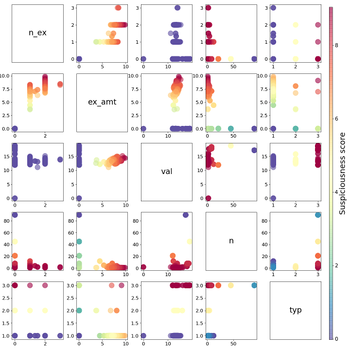
In order to use regression to rank our properties by suspiciousness, we need to score some of our records by hand. So I browsed my dataset, found a few seemingly egregious examples, and gave them high scores (I chose zero through ten, with ten being very suspicious). Then I found a few records I wanted to be sure to ignore and gave them a low score. With a few of these hand labeled records, I was ready to build my Lasso model.

Visual description of a Lasso regression model. In this scatter matrix, each feature is plotted against the other features, forming a scatter plot for each combination. For example, the bottom left plot shows "property type" on the y-axis vs. "number of exemptions" on the x-axis. Points are colored by the suspiciousness scores obtained by the combination of the two features. Red dots are the most suspicious; dark blue/purple dots are the least suspicious.
There's a major benefit to using regression models: the weights they assign to your input variables are straightforward to understand. Other ML models are basically black boxes. This is so much the case that there's an entire subfield of ML dedicated to building models that can interpret other models. In journalism, we need to quickly check our model's assumptions and biases. Regression gives us a way to do this.
As an example, here's a breakdown of a Lasso model I trained:
           Lasso model explanation

Feature                    Importance
_______________________________________________
Property type          =>  2.3802236455789316
Total exemption amount =>  0.9168560761627526
Number of properties   => -0.052699999380756465
Number of exemptions   =>  Ignored
Valuation              =>  Ignored


                (Prop type * 2.38)
              - (No. props * 0.05)
       + (Total exempt amt * 0.91)
       ===========================
                    Suspiciousness
In general, this model thought "property type" was the most important feature. But it found records with large numbers of properties owned by a single person worth ignoring. This is because the data lacked details like unit/apartment numbers, so searches returned properties for every apartment in a complex. Because of this, the regression model decided to ignore buckets with huge numbers of properties. The total exemption amount would bring up a record's suspiciousness score, while number of exemptions and valuation were ignored.
In regression, each of these weights gets multiplied by the corresponding value from each record. When summed, we get a suspiciousness score for each record. Data in, data out.
There were three property types: 1, 2 and 3. Since there were very few type 2 and 3 properties in my dataset, it was important to look into them. Anything rare in a dataset usually is worth looking into. Some of the addresses pointed to large apartment complexes. Unfortunately, our data was lacking apartment or suite numbers, so searches for these properties would bring back every unit in the building. If a bucket contained a lot of properties, it was probably because of a search result like this. Total exemption amount was also an important variable. In this case, my model figured out that "number of exemptions" and "valuation" were directly related to the "total exemption amount". Because of this, we only needed the total exemption amount and could ignore the other two variables.
Using this, I was able to run my grouped records through the trained Lasso regression model and get back a ranked list of records. The top scoring records being the most likely to be worth manual investigative effort.
In one investigation, when the algorithms were done spitting out results, we filed public information requests for hundreds of property tax applications. We got a stack of paper four inches thick that my girlfriend and I carefully spread across our living room floor, cataloged and verified. The Austin Bulldog used this analysis to produce a two-part investigative story about the appraisal district's reluctance to vet tax exemption applications. Hundreds of thousands of dollars in back taxes were reclaimed for taxpayers.
In another investigation, we identified properties that were likely running large, illegal online STRs and getting unwarranted tax breaks. The fallout from this one is still ongoing.
Both investigations wouldn't have been possible without algorithmic assistance. But no matter how many fancy computational methods you use during an investigation, you can never escape the need to go back to the primary, physical sources and meticulously check your work.
Machine learning is just a tool, not magic. It won't do our investigation for us and it won't follow the leads it provides. But when used correctly, it can unlock leads from data and help get us to the part we’re good at: writing stories that expose wrongdoing and effecting change.
